Variational classifier - Parity Classification#
This notebook is adapted from the Pennylane tutorial on variational quantum classifiers. We show how to combine Pennylane’s QML facilities with Covalent to learn the parity function
First we install the required packages.
[1]:
with open("./requirements.txt", "r") as file:
    for line in file:
        print(line.rstrip())
covalent
matplotlib==3.4.3
pennylane==0.25.1
[2]:
# Install required packages
# !pip install -r ./requirements.txt
We import PennyLane, the PennyLane-provided version of NumPy, and an optimizer.
[3]:
import pennylane as qml
from pennylane import numpy as np
import covalent as ct
import matplotlib.pyplot as plt
from pennylane.optimize import NesterovMomentumOptimizer
[4]:
dev = qml.device("default.qubit", wires=4)
Variational classifiers usually define a “layer” or “block”, which is an elementary circuit architecture that gets repeated to build the variational circuit. We have a quantum circuit which contains some rotation gates with trainable rotation angles. The qubits are also being entangled using circular entanglement.
Our quantum circuit architecture is inspired by Farhi and Neven (2018) as well as Schuld et al. (2018).
[5]:
def layer(W):

    qml.Rot(W[0, 0], W[0, 1], W[0, 2], wires=0)
    qml.Rot(W[1, 0], W[1, 1], W[1, 2], wires=1)
    qml.Rot(W[2, 0], W[2, 1], W[2, 2], wires=2)
    qml.Rot(W[3, 0], W[3, 1], W[3, 2], wires=3)

    qml.CNOT(wires=[0, 1])
    qml.CNOT(wires=[1, 2])
    qml.CNOT(wires=[2, 3])
    qml.CNOT(wires=[3, 0])
We also need a way to encode data inputs x into the circuit, so that the measured output depends on the inputs. We use the BasisState function provided by PennyLane to encode the bit vectors into basis states as follows:
@ct.electron#
Each major step of the workflow is constructed using the ct.electron decorator which transforms a function into an Electron object. Electrons are self-contained building blocks of a Covalent workflow.
We begin by defining some (non-Electron) auxiliary functions.
[6]:
def statepreparation(x):
    qml.BasisState(x, wires=[0, 1, 2, 3])
Now we define the quantum node as a state preparation routine, followed by a repetition of the layer structure. Borrowing from machine learning, we call the parameters weights.
[7]:
@qml.qnode(dev)
def circuit(weights, x):

    statepreparation(x)

    for W in weights:
        layer(W)

    return qml.expval(qml.PauliZ(0))
The circuit takes the input state x and then applies the quantum model. Finally it applies Z measurement and returns the result to classical training system.
Here the weights are the trainable parameters which are being trained based on the cost function.
[8]:
def variational_classifier(weights, bias, x):
    return circuit(weights, x) + bias
We use a mean square loss function as a cost function.
[9]:
def square_loss(labels, predictions):
    loss = 0
    for l, p in zip(labels, predictions):
        loss = loss + (l - p) ** 2

    loss = loss / len(labels)
    return loss
We check for accuracy by comparing the true parity values with the prediction.
[10]:
def accuracy(labels, predictions):

    loss = 0
    for l, p in zip(labels, predictions):
        if abs(l - p) < 1e-5:
            loss = loss + 1
    loss = loss / len(labels)

    return loss
Cost
We use the standard square loss that measures the distance between target labels and model predictions.
[11]:
def cost(weights, bias, X, Y):
    predictions = [variational_classifier(weights, bias, x) for x in X]
    return square_loss(Y, predictions)
Optimization
We use a NesterovMomentumOptimizer to perform the training optimization. The advantage of this optimizer from using Gradient descent is that, it a minimum loss path has been found, it uses the momentum to speed up the learning process.
The parity dataset can be downloaded here and should be placed in the subfolder ./assets/parity.txt.
[12]:
@ct.electron
def get_optimizer():
    return NesterovMomentumOptimizer(0.25)
We initialize the variables randomly (but fix a seed for reproducibility). The first variable in the list is used as a bias, while the rest is fed into the gates of the variational circuit.
[13]:
@ct.electron(executor="local")
def weights_bias_init(num_layers, num_qubits):
    weights_init = 0.01 * np.random.randn(num_layers, num_qubits, 3, requires_grad=True)
    bias_init = np.array(0.0, requires_grad=True)
    return weights_init, bias_init
Note: The “local” executor is used for this Electron to work around a serialization bug in the default Dask-based executor. This issue will be addressed in a later release.
We now perform the training for 25 iterations with a batch size of 5. The model’s output is converted to -1 if it’s 0 and +1 if it’s 1 so as to match the dataset.
[14]:
@ct.electron
def training(opt, weights, bias, epochs, batch_size, X, Y, num_layers, num_qubits, cost):
    # weights,bias = weights_bias_init(num_layers,num_qubits)
    training_steps = []
    cost_steps = []
    accuracy_steps = []
    for it in range(epochs):
        batch_index = np.random.randint(0, len(X), (batch_size,))
        X_batch = X[batch_index]
        Y_batch = Y[batch_index]
        weights, bias, _, _ = opt.step(cost, weights, bias, X_batch, Y_batch)

        # Compute accuracy
        predictions = [np.sign(variational_classifier(weights, bias, x)) for x in X]
        acc = accuracy(Y, predictions)
        training_steps.append(it)
        cost_steps.append(cost(weights, bias, X, Y))
        accuracy_steps.append(acc)

        print(
            "Iter: {:5d} | Cost: {:0.7f} | Accuracy: {:0.7f} ".format(
                it + 1, cost(weights, bias, X, Y), acc
            )
        )

    return weights, bias, training_steps, cost_steps, accuracy_steps
We create a workflow using covalent and distribute the loads
@ct.lattice
We now construct a Lattice tying together the different Electrons comprising the workflow.
[15]:
@ct.lattice
def workflow(epochs, num_layers, num_qubits, X, Y):
    opt = get_optimizer()
    weights, bias = weights_bias_init(num_layers, num_qubits)
    batch_size = 5
    weights, bias, training_steps, cost_steps, accuracy_steps = training(
        opt, weights, bias, epochs, batch_size, X, Y, num_layers, num_qubits, cost
    )
    return weights, bias, training_steps, cost_steps, accuracy_steps
[16]:
data = np.loadtxt("assets/parity.txt")
X = np.array(data[:, :-1], requires_grad=False)
Y = np.array(data[:, -1], requires_grad=False)
Y = Y * 2 - np.ones(len(Y))  # shift label from {0, 1} to {-1, 1}

for i in range(5):
    print("X = {}, Y = {: d}".format(X[i], int(Y[i])))

print("...")
X = [0. 0. 0. 0.], Y = -1
X = [0. 0. 0. 1.], Y =  1
X = [0. 0. 1. 0.], Y =  1
X = [0. 0. 1. 1.], Y = -1
X = [0. 1. 0. 0.], Y =  1
...
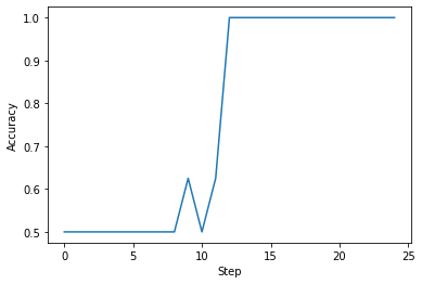
We dispatch the workflow. The results are obtained from the covalent and plotted:
[17]:
dispatch_id = ct.dispatch(workflow)(X=X, Y=Y, epochs=25, num_layers=2, num_qubits=4)
result = ct.get_result(dispatch_id=dispatch_id, wait=True)
weights, bias, training_steps, cost_steps, accuracy_steps = result.result
[18]:
plt.plot(training_steps, accuracy_steps)
plt.xlabel("Step")
plt.ylabel("Accuracy")
plt.show()
References