Iris classification

This section of the tutorial makes use of the Iris Dataset which contains the features of the flowers needed to perform a classification task and get the corresponding flower names. We use amplitude encoding for encoding the features in the dataset and use a Quantum machine learning model to perform the classification.

with open("./requirements.txt", "r") as file:
    for line in file:
        print(line.rstrip())

covalent
matplotlib==3.4.3
pennylane==0.25.1
pennylane-sf==0.20.1

# Install necessary packages
# !pip install -r ./requirements.txt

import pennylane as qml
from pennylane import numpy as np
import covalent as ct
import matplotlib.pyplot as plt
from pennylane.optimize import NesterovMomentumOptimizer

We use the Pennylane quantum simulator with 2 qubits to encode real-valued vectors into the amplitudes of a quantum state.

dev = qml.device("default.qubit", wires=2)

Next, we perform the amplitude encoding of the features by first converting the features to angles. We then use a state preparation circuit and feed in those angles and perform the amplitude encoding of the features.

As noted in the original Pennylane tutorial, the circuit is coded according to the scheme in Möttönen, et al. (2004), or as presented for positive vectors only in Schuld and Petruccione (2018). Additionally, controlled Y-axis rotations are decomposed into more basic circuits following similar steps in Nielsen and Chuang (2010).

@ct.electron
def get_angles(x):

    beta0 = 2 * np.arcsin(np.sqrt(x[1] ** 2) / np.sqrt(x[0] ** 2 + x[1] ** 2 + 1e-12))
    beta1 = 2 * np.arcsin(np.sqrt(x[3] ** 2) / np.sqrt(x[2] ** 2 + x[3] ** 2 + 1e-12))
    beta2 = 2 * np.arcsin(
        np.sqrt(x[2] ** 2 + x[3] ** 2) / np.sqrt(x[0] ** 2 + x[1] ** 2 + x[2] ** 2 + x[3] ** 2)
    )

    return np.array([beta2, -beta1 / 2, beta1 / 2, -beta0 / 2, beta0 / 2])

def statepreparation(a):
    qml.RY(a[0], wires=0)

    qml.CNOT(wires=[0, 1])
    qml.RY(a[1], wires=1)
    qml.CNOT(wires=[0, 1])
    qml.RY(a[2], wires=1)

    qml.PauliX(wires=0)
    qml.CNOT(wires=[0, 1])
    qml.RY(a[3], wires=1)
    qml.CNOT(wires=[0, 1])
    qml.RY(a[4], wires=1)
    qml.PauliX(wires=0)

def layer(W):
    qml.Rot(W[0, 0], W[0, 1], W[0, 2], wires=0)
    qml.Rot(W[1, 0], W[1, 1], W[1, 2], wires=1)
    qml.CNOT(wires=[0, 1])

In essence, the variational classifier model contains the state preparation circuit and the quantum model. The measurement is performed using Z-measurement and the result is passed to a classical training system.

@qml.qnode(dev)
def circuit(weights, angles):
    statepreparation(angles)

    for W in weights:
        layer(W)

    return qml.expval(qml.PauliZ(0))

We use a mean square loss function as a cost function.

@ct.electron
def square_loss(labels, predictions):
    loss = 0
    for l, p in zip(labels, predictions):
        loss = loss + (l - p) ** 2

    loss = loss / len(labels)
    return loss

@ct.electron
def variational_classifier(weights, bias, angles):
    return circuit(weights, angles) + bias

Cost

In supervised learning, the cost function is usually the sum of a loss function and a regularizer. We use the standard square loss that measures the distance between target labels and model predictions.

@ct.electron
def cost(weights, bias, features, labels):
    predictions = [variational_classifier(weights, bias, f) for f in features]
    return square_loss(labels, predictions)

@ct.electron
def load_features(data):
    # pad the vectors to size 2^2 with constant values
    X = data[:, 0:2]
    print("First X sample (original)  :", X[0])

    padding = 0.3 * np.ones((len(X), 1))
    X_pad = np.c_[np.c_[X, padding], np.zeros((len(X), 1))]
    print("First X sample (padded)    :", X_pad[0])

    # normalize each input
    normalization = np.sqrt(np.sum(X_pad**2, -1))
    X_norm = (X_pad.T / normalization).T
    print("First X sample (normalized):", X_norm[0])

    # angles for state preparation are new features
    features = np.array([get_angles(x) for x in X_norm], requires_grad=False)
    Y = data[:, -1]
    return features, Y, X, X_norm, X_pad

Data

Now, we load the Iris dataset and perform the amplitude encoding. We then pass it to a model.

The Iris dataset can be downloaded here and should be placed in the subfolder ./iris_classes1and2_scaled.txt.

data = np.loadtxt("assets/iris_classes1and2_scaled.txt")

features, Y, X, X_norm, X_pad = load_features(data)

print("First features sample      :", features[0])

First X sample (original)  : [0.4  0.75]
First X sample (padded)    : [0.4  0.75 0.3  0.  ]
First X sample (normalized): [0.44376016 0.83205029 0.33282012 0.        ]
First features sample      : [ 0.67858523 -0.          0.         -1.080839    1.080839  ]

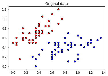
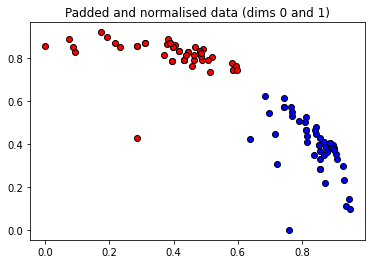
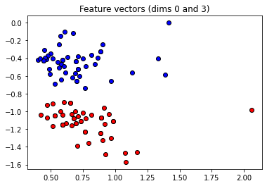
These angles are our new features, which is why we have renamed X to “features” above. Let’s plot the stages of preprocessing and play around with the dimensions (dim1, dim2). Some of them still separate the classes well, while others are less informative.

import matplotlib.pyplot as plt

plt.figure()
plt.scatter(X[:, 0][Y == 1], X[:, 1][Y == 1], c="b", marker="o", edgecolors="k")
plt.scatter(X[:, 0][Y == -1], X[:, 1][Y == -1], c="r", marker="o", edgecolors="k")
plt.title("Original data")
plt.show()

plt.figure()
dim1 = 0
dim2 = 1
plt.scatter(X_norm[:, dim1][Y == 1], X_norm[:, dim2][Y == 1], c="b", marker="o", edgecolors="k")
plt.scatter(X_norm[:, dim1][Y == -1], X_norm[:, dim2][Y == -1], c="r", marker="o", edgecolors="k")
plt.title("Padded and normalised data (dims {} and {})".format(dim1, dim2))
plt.show()

plt.figure()
dim1 = 0
dim2 = 3
plt.scatter(
    features[:, dim1][Y == 1], features[:, dim2][Y == 1], c="b", marker="o", edgecolors="k"
)
plt.scatter(
    features[:, dim1][Y == -1], features[:, dim2][Y == -1], c="r", marker="o", edgecolors="k"
)
plt.title("Feature vectors (dims {} and {})".format(dim1, dim2))
plt.show()

To monitor the generalization performance, we split the dataset into two subsets namely train set and validation set. The train set contains 75% data and the validation set contains 25% data.

@ct.electron
def train_val_split(features, Y):
    np.random.seed(0)
    num_data = len(Y)
    num_train = int(0.75 * num_data)
    index = np.random.permutation(range(num_data))
    feats_train = features[index[:num_train]]
    Y_train = Y[index[:num_train]]
    feats_val = features[index[num_train:]]
    Y_val = Y[index[num_train:]]
    return feats_train, Y_train, feats_val, Y_val, index, num_train

feats_train, Y_train, feats_val, Y_val, index, num_train = train_val_split(features, Y)
X_train = X[index[:num_train]]
X_val = X[index[num_train:]]

We check for accuracy by comparing the true parity values with the prediction.

@ct.electron
def accuracy(labels, predictions):

    loss = 0
    for l, p in zip(labels, predictions):
        if abs(l - p) < 1e-5:
            loss = loss + 1
    loss = loss / len(labels)

    return loss

We initialize the variables randomly (but fix a seed for reproducibility). The first variable in the list is used as a bias, while the rest is fed into the gates of the variational circuit.

@ct.electron
def weights_bias_init(num_qubits, num_layers):
    weights_init = 0.01 * np.random.randn(num_layers, num_qubits, 3, requires_grad=True)
    bias_init = np.array(0.0, requires_grad=True)
    return weights_init, bias_init

Optimization

We use a NesterovMomentumOptimizer to perform the training optimization. The advantage of using the NesterovMomentumOptimizier compared to using Gradient Descent is that when a minimum loss path is found, the NesterovMomentumOptimizer uses the momentum to speed up the learning process.

def get_optimizer():
    return NesterovMomentumOptimizer(0.005)

We also optimize the cost.

@ct.electron
def training(
    iterations,
    batch_size,
    weights,
    bias,
    num_train,
    feats_train,
    Y_train,
    opt,
    feats_val,
    Y_val,
    Y,
):
    # print("beginning")
    training_steps = []
    accuracy_steps_train = []
    accuracy_steps_val = []
    weights_init = weights
    bias_init = bias
    for it in range(iterations):
        batch_index = np.random.randint(0, num_train, (batch_size,))
        # print("Here")
        feats_train_batch = feats_train[batch_index]
        Y_train_batch = Y_train[batch_index]
        # print("Here1")
        weights_init, bias_init, _, _ = opt.step(
            cost, weights_init, bias_init, feats_train_batch, Y_train_batch
        )
        # print("Here2")
        training_steps.append(it)
        # Compute predictions on train and validation set
        predictions_train = [
            np.sign(variational_classifier(weights_init, bias_init, f)) for f in feats_train
        ]
        predictions_val = [
            np.sign(variational_classifier(weights_init, bias_init, f)) for f in feats_val
        ]
        # print("Here3")
        # Compute accuracy on train and validation set
        acc_train = accuracy(Y_train, predictions_train)
        acc_val = accuracy(Y_val, predictions_val)
        # print("Here4")
        accuracy_steps_train.append(acc_train)
        accuracy_steps_val.append(acc_val)
        # print("Here5")
        print(
            "Iter: {:5d} | Cost: {:0.7f} | Acc train: {:0.7f} | Acc validation: {:0.7f} "
            "".format(it + 1, cost(weights, bias, features, Y), acc_train, acc_val)
        )
    return weights_init, bias_init, training_steps, accuracy_steps_train, accuracy_steps_val

Note: In Covalent, a function can be decorated as a lattice or workflow by using``@ct.lattice``. The decorated function, i.e., the lattice contains electrons which are called as normal functions.

@ct.lattice(executor="local")
def workflow(
    iterations, num_train, num_layers, num_qubits, feats_train, Y_train, feats_val, Y_val, Y
):
    opt = get_optimizer()
    weights, bias = weights_bias_init(num_layers, num_qubits)
    batch_size = 10
    weights_init, bias_init, training_steps, accuracy_steps_train, accuracy_steps_val = training(
        iterations=iterations,
        batch_size=batch_size,
        weights=weights,
        bias=bias,
        num_train=num_train,
        feats_train=feats_train,
        Y_train=Y_train,
        opt=opt,
        feats_val=feats_val,
        Y_val=Y_val,
        Y=Y,
    )
    return weights_init, bias_init, training_steps, accuracy_steps_train, accuracy_steps_val

The workflow is being dispatched and we can see progress in Covalent dashboard. The results are obtained from the covalent and plotted

Note: The “local” executor is used for the lattice to work around a serialization bug in the default Dask-based executor. This issue will be addressed in a later release.

dispatch_id = ct.dispatch(workflow)(
    feats_train=feats_train,
    Y_train=Y_train,
    feats_val=feats_val,
    Y_val=Y_val,
    iterations=80,
    num_qubits=2,
    num_layers=6,
    num_train=num_train,
    Y=Y,
)
result = ct.get_result(dispatch_id=dispatch_id, wait=True)
weights, bias, training_steps, cost_steps, accuracy_steps = result.result

print(f"Workflow completion status: {result.status}")

Workflow completion status: COMPLETED

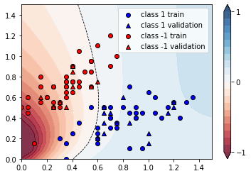
We can plot the continuous output of the variational classifier for the first two dimensions of the Iris data set.

plt.figure()
cm = plt.cm.RdBu

# make data for decision regions
xx, yy = np.meshgrid(np.linspace(0.0, 1.5, 20), np.linspace(0.0, 1.5, 20))
X_grid = [np.array([x, y]) for x, y in zip(xx.flatten(), yy.flatten())]

# preprocess grid points like data inputs above
padding = 0.3 * np.ones((len(X_grid), 1))
X_grid = np.c_[np.c_[X_grid, padding], np.zeros((len(X_grid), 1))]  # pad each input
normalization = np.sqrt(np.sum(X_grid**2, -1))
X_grid = (X_grid.T / normalization).T  # normalize each input
features_grid = np.array(
    [get_angles(x) for x in X_grid]
)  # angles for state preparation are new features
predictions_grid = [variational_classifier(weights, bias, f) for f in features_grid]
Z = np.reshape(predictions_grid, xx.shape)

# plot decision regions
cnt = plt.contourf(xx, yy, Z, levels=np.arange(-1, 1.1, 0.1), cmap=cm, alpha=0.8, extend="both")
plt.contour(xx, yy, Z, levels=[0.0], colors=("black",), linestyles=("--",), linewidths=(0.8,))
plt.colorbar(cnt, ticks=[-1, 0, 1])

# plot data
plt.scatter(
    X_train[:, 0][Y_train == 1],
    X_train[:, 1][Y_train == 1],
    c="b",
    marker="o",
    edgecolors="k",
    label="class 1 train",
)
plt.scatter(
    X_val[:, 0][Y_val == 1],
    X_val[:, 1][Y_val == 1],
    c="b",
    marker="^",
    edgecolors="k",
    label="class 1 validation",
)
plt.scatter(
    X_train[:, 0][Y_train == -1],
    X_train[:, 1][Y_train == -1],
    c="r",
    marker="o",
    edgecolors="k",
    label="class -1 train",
)
plt.scatter(
    X_val[:, 0][Y_val == -1],
    X_val[:, 1][Y_val == -1],
    c="r",
    marker="^",
    edgecolors="k",
    label="class -1 validation",
)

plt.legend()
plt.show()

References

• https://pennylane.ai/qml/demos/tutorial_variational_classifier.html

• https://covalent.readthedocs.io/en/latest/index.html