Linear and convolutional autoencoders

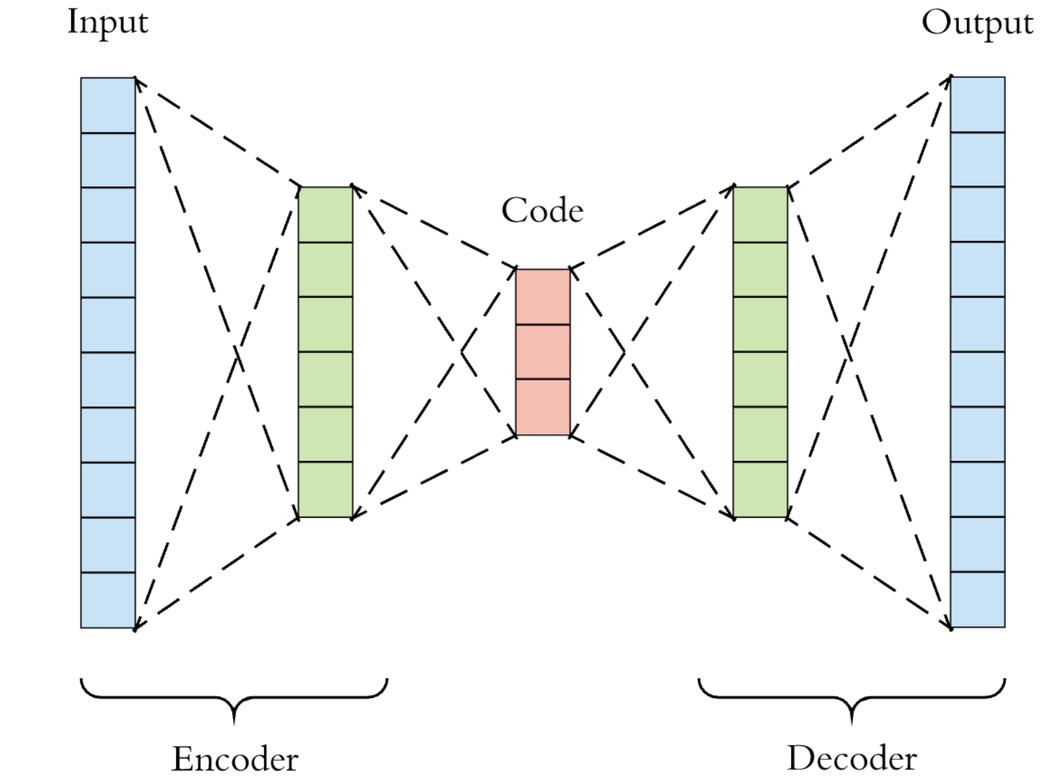
An autoencoder is a neural network that can be used to encode and decode data. The general structure of an autoencoder is shown in the figure below. It consists of two parts: an encoder and a decoder. The encoder compresses the input data into a lower dimensional representation (“code” in the schematic below, which is often referred to as the latent space representation) by extracting the most salient features of the data, while the decoder reconstructs the input data from the compressed representation. Therefore, autoencoder is often used for dimensionality reduction. In this tutorial, our goal is to compare the performance of two types of autoencoders, a linear autoencoder and a convolutional autoencoder, on reconstructing the Fashion-MNIST images. With the help of Covalent, we will see how to break a complex workflow into smaller and more manageable tasks, which allows users to track the task dependencies and execution results of individual steps. Another advantage of Covalent is its ability to auto-parallelize the execution of subtasks.

Building the autoencoders

We will build the two types of autoencoders in PyTorch. The linear autoencoder is built on the Linear layers, while the convolutional autoencoder is built on the Conv2d layers. Let us first install all the necessary dependencies for this tutorial.

with open("./requirements.txt", "r") as file:
    for line in file:
        print(line.rstrip())

covalent
matplotlib==3.5.1
numpy==1.23.2
torch==1.13.1
torchvision==0.14.1

# Installing required packages
# !pip install -r ./requirements.txt

We can then start the Covalent UI and the local dispatcher server by running !covalent start. Next, we import the following modules:

import torch
import torch.nn as nn
import torch.optim as optim
import matplotlib.pyplot as plt
import numpy as np
from torchvision import datasets, transforms
import covalent as ct

The linear and convolutional autoencoders are implemented as classes inheriting from the nn.Module class in PyTorch. We will define two functions called create_linear_ae and create_conv_ae to create the linear and convolutional autoencoders, respectively, and add the electron decorator on top to make them part of the Covalent workflow. The advantage of doing this is that various parts of the autoencoder network such as the number of hidden layers and their sizes can be parameterized by the user for experimentation. For this tutorial, we will use a fixed architecture for each of them for the sake of simplicity.

In the case of a linear autoencoder, we will use four hidden layers in the encoder. Between each layer the ReLU activation function is applied. The decoder is essentially the “inverse” of the encoder, and we will use the same architecture for it except at the end an additional Sigmoid activation function is applied. The choice of this activation function depends on the range of the pixel intensity in the original input data. Note that the Fashion-MNIST dataset contains 28x28-pixel gray-scale images, so the input dimension of each image is 28x28x1. The compressed images generated by the encoder in this case would have dimension 3x3x1 in this case. In addition,

@ct.electron
def create_linear_ae():
    class LinearAutoencoder(nn.Module):
        """Autoencoder with 4 hidden layers."""

        def __init__(self):
            super(LinearAutoencoder, self).__init__()
            self.encoder = nn.Sequential(
                nn.Linear(28 * 28, 128),  # input size = 784 -> hidden size = 128
                nn.ReLU(True),
                nn.Linear(128, 64),  # hidden size = 128 -> hidden size = 64
                nn.ReLU(True),
                nn.Linear(64, 12),  # hidden size = 64 -> hidden size = 12
                nn.ReLU(True),
                nn.Linear(12, 3),  # hidden size = 12 -> output size = 3
            )
            self.decoder = nn.Sequential(
                nn.Linear(3, 12),  # input size = 3 -> hidden size = 12
                nn.ReLU(True),
                nn.Linear(12, 64),  # hidden size = 12 -> hidden size = 64
                nn.ReLU(True),
                nn.Linear(64, 128),  # hidden size = 64 -> hidden size = 128
                nn.ReLU(True),
                nn.Linear(128, 28 * 28),  # hidden size = 128 -> output size = 784
                nn.Sigmoid(),  # output with pixel intensity in [0,1]
            )

        def forward(self, x):
            encoded = self.encoder(x)
            decoded = self.decoder(encoded)
            return decoded

    return LinearAutoencoder()

For the convolutional autoencoder, we will use three hidden layers. Each convolutional layer except for the last one in the encoder will use the Conv2d construction with a kernel size of 3x3, a stride of 1, and a padding of 1, followed by a ReLU activation function. The decoder will use the ConvTranspose2d layers to reverse the action of the Conv2d layers in the encoder, followed by a Sigmoid activation function.

def create_conv_ae():
    class ConvAutoencoder(nn.Module):
        """Autoencoder with 3 hidden layers."""

        def __init__(self):
            super(ConvAutoencoder, self).__init__()
            self.encoder = nn.Sequential(
                nn.Conv2d(
                    1, 16, 3, stride=2, padding=1
                ),  # input size = 1x28x28 -> hidden size = 16x14x14
                nn.ReLU(True),
                nn.Conv2d(
                    16, 32, 3, stride=2, padding=1
                ),  # hidden size = 16x14x14 -> hidden size = 32x7x7
                nn.ReLU(True),
                nn.Conv2d(32, 64, 7),  # hidden size = 32x7x7 -> hidden size = 64x1x1
            )

            self.decoder = nn.Sequential(
                nn.ConvTranspose2d(64, 32, 7),  # input size = 64x1x1 -> hidden size = 32x7x7
                nn.ReLU(True),
                nn.ConvTranspose2d(
                    32, 16, 3, stride=2, padding=1, output_padding=1
                ),  # hidden size = 32x7x7 -> hidden size = 16x14x14
                nn.ReLU(True),
                nn.ConvTranspose2d(
                    16, 1, 3, stride=2, padding=1, output_padding=1
                ),  # hidden size = 16x14x14 -> hidden size = 1x28x28
                nn.Sigmoid(),  # output with pixels in [0,1]
            )

        def forward(self, x):
            encoded = self.encoder(x)
            decoded = self.decoder(encoded)
            return decoded

    return ConvAutoencoder()

Creating the workflow

Let us now build a workflow that can encompass both autoencoders. Overall, the workflow consists of five tasks. We begin by creating a data_loader that loads the data from the Fashion-MNIST dataset, along with custom preprocessing if necessary. We will add the electron decorator on this function, making it a subtask in the Covalent workflow.

@ct.electron
def data_loader(
    batch_size: int,
    train: bool,
    download: bool = True,
    shuffle: bool = False,
    transform: transforms.Compose = None,
) -> torch.utils.data.DataLoader:
    """
    Loads the Fashion MNIST dataset.

    Args:
        batch_size: The batch size.
        train: Whether to load the training or test set.
        download: Whether to download the dataset.
        shuffle: Whether to shuffle the dataset.
        transform: A transform to apply to the dataset.

    Returns:
        A DataLoader for the Fashion MNIST dataset.
    """
    if transform is None:
        transform = transforms.Compose([transforms.ToTensor()])

    dataset = datasets.FashionMNIST("./data", train=train, download=download, transform=transform)

    return torch.utils.data.DataLoader(dataset, batch_size=batch_size, shuffle=shuffle)

Then we define the training process over multiple epochs. To optimize the autoencoders, we choose the Adam optimizer as our optimizer and the mean squared error (MSE) between the original and reconstructed images as the reconstruction loss. The MSE is defined as \begin{equation} \text{MSE}(\vec W) = \frac{1}{n}\sum_{i=1}^n \lvert x_i - \hat x_i(\vec W) \rvert^2, \end{equation}

where \(n\) is the number of pixels in any input image, \(x_i\) and \(\hat x_i\) correspond to the individual pixels in the original and reconstructed images, respectively, and the vector \(\vec W\) contains the weights in the autoencoder networks that we will try to optimize. During training, we will keep track of the reconstruction loss after each epoch. We will also log the output images after a certain number of epochs specified by the log_interval.

@ct.electron
def train_model(
    model: nn.Module,
    lr: float,
    data_loader: torch.utils.data.DataLoader,
    epochs: int,
    log_interval: int,
):
    """
    Trains the given model on the Fashion MNIST dataset.

    Args:
        model: A PyTorch model.
        lr: The learning rate.
        data_loader: A DataLoader for the Fashion MNIST dataset.
        epochs: The number of epochs to train for.
        log_interval: The number of epochs to wait before logging in the outputs.

    Returns:
        train_loss: A list of training losses for each epoch.
        outputs: Contains epoch number, the original image, and the reconstructed image at each training step.
        model: The trained model.
    """
    optimizer = optim.Adam(model.parameters(), lr=lr)
    model.train()
    outputs = []
    train_loss = []
    print(f"Training {model.__class__.__name__}")
    for epoch in range(1, epochs + 1):
        running_loss = 0
        for (data, _) in data_loader:
            if model.__class__.__name__ == "LinearAutoencoder":
                data = data.view(data.size(0), -1)
            recon = model(data)
            loss = nn.MSELoss()(recon, data)  # mean squared error loss
            optimizer.zero_grad()
            loss.backward()
            optimizer.step()
            running_loss += loss.item()
        loss = running_loss / len(data_loader)
        train_loss.append(loss)
        if epoch % log_interval == 0:
            outputs.append((epoch, data, recon))
            print(f"Epoch {epoch}, loss: {loss}")
    return train_loss, outputs, model

After the training is complete, we will test the performance of our autoencoders on the test set and compare the average test loss with the training losses.

@ct.electron
def test_model(
    model: nn.Module,
    data_loader: torch.utils.data.DataLoader,
):
    """
    Tests the given model on the Fashion MNIST dataset.

    Args:
        model: A PyTorch model.
        data_loader: A DataLoader for the Fashion MNIST dataset.

    Returns:
        avg_test_loss: The average loss for the test set.
    """
    model.eval()
    test_loss = 0
    with torch.no_grad():
        for (data, _) in data_loader:
            if model.__class__.__name__ == "LinearAutoencoder":
                data = data.view(data.shape[0], -1)
            recon = model(data)
            loss = nn.MSELoss()(recon, data)  # mean squared error loss
            test_loss += loss.item()
    avg_test_loss = test_loss / len(data_loader)
    print(f"Average test loss: {avg_test_loss}")
    return avg_test_loss

With the above subtasks properly set up, we can bundle them into one single workflow that trains and tests a given autoencoder (linear or convolutional). Since we want to compare the performance of the two architectures, we will make this workflow an electron instead of a lattice for now. Alternatively, one can use the lattice decorator for the following workflow and then make it a sublattice of a larger workflow by using ct.electron(experiment).

@ct.electron
def experiment(
    model: nn.Module,
    epochs: int,
    log_interval: int,
    batch_size_train: int = 64,
    batch_size_test: int = 1000,
    lr: float = 1e-3,
):
    """
    Workflow of training and testing a given autoencoder (linear or convolutional) on the Fashion MNIST dataset.

    Args:
        model: A PyTorch model.
        epochs: The number of epochs to train for.
        log_interval: The number of epochs to wait before logging in the outputs.
        batch_size_train: The batch size for the training set.
        batch_size_test: The batch size for the test set.
        lr: The learning rate.

    Returns:
        train_loss: The training loss at each epoch.
        avg_test_loss: The average loss for the test set.
        outputs: Contains epoch number, the original image, and the reconstructed image at each training step.
    """
    train_loader = data_loader(batch_size=batch_size_train, train=True)
    test_loader = data_loader(batch_size=batch_size_test, train=False)

    train_loss, outputs, model = train_model(
        model=model,
        lr=lr,
        data_loader=train_loader,
        epochs=epochs,
        log_interval=log_interval,
    )
    avg_test_loss = test_model(model=model, data_loader=test_loader)

    return train_loss, avg_test_loss, outputs

Finally we will create the full workflow that runs both autoencoders in parallel with the help of Covalent.

@ct.lattice
def run_experiments(
    models: list,
    epochs: int,
    log_interval: int,
    batch_size_train: int = 64,
    batch_size_test: int = 1000,
    lr: float = 1e-3,
):
    """
    Run experiments of training and testing a series of autoencoders on the Fashion MNIST dataset.

    Args:
        models: A list of PyTorch models.
        epochs: The number of epochs to train for.
        log_interval: The number of epochs to wait before logging in the outputs.
        batch_size_train: The batch size for the training set.
        batch_size_test: The batch size for the test set.
        lr: The learning rate.

    Returns:
        train_loss: The training loss at each epoch.
        avg_test_loss: The average loss for the test set.
        outputs: Contains epoch number, the original image, and the reconstructed image at each training step.
    """
    train_losses = []
    avg_test_losses = []
    full_outputs = []
    for model in models:
        train_loss, avg_test_loss, outputs = experiment(
            model=model,
            epochs=epochs,
            log_interval=log_interval,
            batch_size_train=batch_size_train,
            batch_size_test=batch_size_test,
            lr=lr,
        )
        train_losses.append(train_loss)
        avg_test_losses.append(avg_test_loss)
        full_outputs.append(outputs)

    return train_losses, avg_test_losses, full_outputs

Linear vs. convolutional autoencoders

We will now run the full experiments and compare the performance of the linear and convolutional autoencoders.

dispatch_id = ct.dispatch(run_experiments)(
    models=[create_linear_ae(), create_conv_ae()], epochs=50, log_interval=10
)
results = ct.get_result(dispatch_id=dispatch_id, wait=True)

train_losses, avg_test_losses, full_outputs = results.result

Here is a snapshot of the workflow on the Covalent UI (http://localhost:48008):

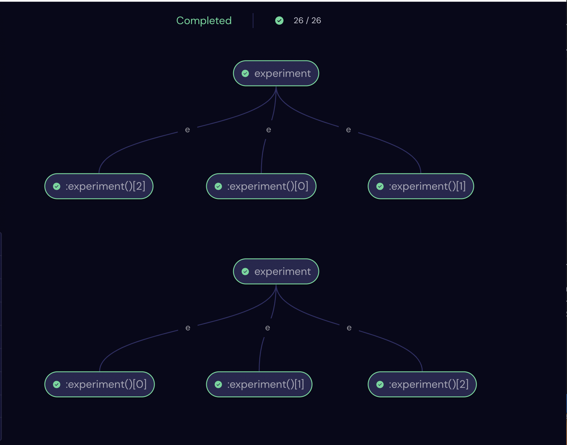
Let us inspect the full training history for both autoencoders, which was saved during the experiments.

fig, axes = plt.subplots(1, 2, figsize=(12, 5), facecolor="w")
axes[0].plot(np.arange(1, len(train_losses[0]) + 1), train_losses[0])
axes[0].set_title("Training loss of linear autoencoder")
axes[0].set_xlabel("Epoch")
axes[0].set_ylabel("Training loss")
axes[1].plot(np.arange(1, len(train_losses[1]) + 1), train_losses[1])
axes[1].set_title("Training loss of convolutional autoencoder")
axes[1].set_xlabel("Epoch")
axes[1].set_ylabel("Training loss")
fig.tight_layout()
plt.show()

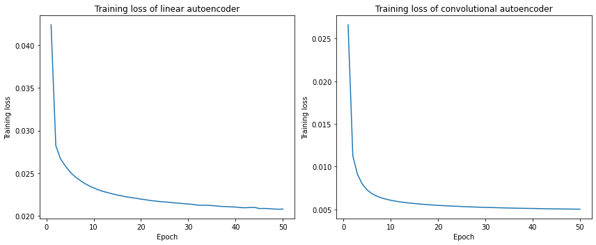
We can print out the final training loss and the average test loss for both autoencoders for comparison.

print(f"Final train loss of linear autoencoder: {train_losses[0][-1]}")
print(f"Final train loss of convolutional autoencoder: {train_losses[1][-1]}")
print(f"Average test loss of linear autoencoder: {avg_test_losses[0]}")
print(f"Average test loss of convolutional autoencoder: {avg_test_losses[1]}")

Final train loss of linear autoencoder: 0.020817029861800833
Final train loss of convolutional autoencoder: 0.005023478609777844
Average test loss of linear autoencoder: 0.02144053615629673
Average test loss of convolutional autoencoder: 0.0052970537915825846

There are a few key takeaways from the above results: 1) For both autoencoders, the training loss decreases significantly with an increasing number of epochs, indicating that the training was successful. 2) The average test loss for 1000 images is about the same as the final training loss. This means that both autoencoders have pretty good generalizability. 3) The loss of the the convolutional autoencoder is just about 1/4 that of the linear autoencoder after 50 epochs, even when the convolutional autoencoder has one fewer hidden layer than its linear counterpart. This is expected since the convolutional neural network is more complex and generally performs better with image data. However, it also took a longer time to optimize the convolutional model under the same number of epochs.

Lastly, we also want to display a few image samples at different phases of training to help us visualize how the reconstructed images from both autoencoders compare with the original ones. We can also directly compare the results of reconstruction based on the linear and convolutional autoencoders.

def plot_outputs(full_outputs: list):
    """
    Plots the output images (original, reconstruction from linear AE,
    and reconstruction from convolutional AE) of the workflow.

    Args:
        full_outputs: The full outputs of the workflow.
    """
    outputs_linear = full_outputs[0]
    outputs_conv = full_outputs[1]
    for i in range(len(outputs_linear)):
        plt.figure(figsize=(12, 6), facecolor="w")
        plt.gray()
        plt.suptitle(f"Epoch {outputs_linear[i][0]}")
        plt.gcf().text(0.02, 0.75, "Original", fontsize=14)
        plt.gcf().text(0.02, 0.48, "Linear", fontsize=14)
        plt.gcf().text(0.02, 0.22, "Convolutional", fontsize=14)
        imgs = outputs_linear[i][1].detach().numpy()  # original images
        recon_linear = outputs_linear[i][2].detach().numpy()  # reconstructed images from linear AE
        recon_conv = outputs_conv[i][2].detach().numpy()  # reconstructed images from conv AE

        for j, item in enumerate(imgs):
            while j < 5:
                plt.subplot(3, 5, j + 1)
                item = item.reshape(-1, 28, 28)
                plt.imshow(item[0])
                plt.axis("off")
                j += 1

        for j, item in enumerate(recon_linear):
            while j < 5:
                plt.subplot(3, 5, j + 6)
                item = item.reshape(-1, 28, 28)
                plt.imshow(item[0])
                plt.axis("off")
                j += 1

        for j, item in enumerate(recon_conv):
            while j < 5:
                plt.subplot(3, 5, j + 11)
                item = item.reshape(-1, 28, 28)
                plt.imshow(item[0])
                plt.axis("off")
                j += 1


plot_outputs(full_outputs)

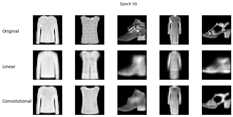
Comparing the reconstructed images from both autoencoders against the original ones, the improvement with increasing number of epochs is pretty obvious. One can also see that the overall reconstruction quality of the linear autoencoder is inferior to that of the convolutional counterpart. This is especially evident at earlier training stages. In most cases of using the linear model, the reconstructed image is only capable of capturing the overall shape of the original objects, while losing a significant amount of details. In comparison, the convolutional model is able to capture much more details of the original images.

Conclusion

In summary, we introduced the concept of autoencoders, constructed two types of autoencoder, linear and convolutional, to reconstruct the Fashion-MNIST images and compared the performance of them. We saw that using Covalent, we were able to break the problem down into a series of subtasks. Moreover, taking advantage of auto-parallelization of the Covalent workflow, we successfully conducted an experiment where we trained and tested both autoencoders at the same time. This feature gives users the flexibility in performing experiments with various models and parameters to even a much larger scale. Overall, we saw that the convolutional architecture performed better than the linear architecture for this task, and that the convolutional reconstruction was able to capture more details of the original images.