Using Covalent with PennyLane for hybrid computation#
PennyLane is a popular Python library for differentiable programming of quantum computers that is well suited for quantum machine learning tasks. In this tutorial, we will demonstrate how to integrate Covalent with PennyLane for a simple hybrid quantum-classical optimization task. The hybrid computation shown here contains three paradigms: 1) continuous-variable quantum computing with qumodes; 2) gate-based quantum computing with qubits; and 3) classical computing. For hybrid tasks like this one as well as more complex use cases, Covalent is able to intelligently schedule the subtasks to be performed on different hardwares and hence helps ease the workload. This tutorial is based on the PennyLane demo: Plugins and Hybrid Computation.
In essence, we will build a simple photonic circuit with two qumodes (i.e., photonic analog of qubits, which are referred to as “wires” in PennyLane) using PennyLane’s Strawberry Fields plugin. The circuit is initialized with the state \(\ket{1,0}\) and contains a beamsplitter with two free parameters \(\theta\) and \(\phi\), which together determine the transmission and reflection amplitudes. In addition, we will build another one-qubit quantum circuit comprising two rotation gates with fixed angles. The goal is to optimize the beamsplitter parameters \((\theta, \phi)\) such that the expectation value of the photon number in the second wire of the photonic circuit is close to the expectation value of measurements of the qubit circuit in the computational basis. In a realistic hybrid implementation, the expectation values would be measured with quantum computers, whereas the optimization would be done on a classical computer. We will see how to use Covalent to manage such hybrid workflows. We refer the reader to the original PennyLane demo for more details on the quantum circuits.
In addition to Covalent, this tutorial uses PennyLane as well as its Strawberry Fields plugin. So we first do the following installations.
[1]:
with open("./requirements.txt", "r") as file:
    for line in file:
        print(line.rstrip())
covalent
pennylane==0.25.1
pennylane-sf==0.20.1
matplotlib==3.4.3
[2]:
# Install necessary packages
# !pip install -r requirements.txt
Then run covalent start in a terminal to start the Covalent server.
Finally, let us import the necessary libraries.
[3]:
import pennylane as qml
from pennylane import numpy as np
import covalent as ct
import matplotlib.pyplot as plt
Construct the workflow#
We can now start constructing our workflow for the hybrid optimization task. First, we initialize two devices with PennyLane, one for the photon-redirection circuit and the other for a qubit-rotation circuit, which is needed for the optimization later.
[3]:
dev_fock = qml.device("strawberryfields.fock", wires=2, cutoff_dim=10)
dev_qubit = qml.device("default.qubit", wires=1)
With the devices initialized, we construct the corresponding quantum nodes by defining the quantum circuits and adding the qnode decorator onto them. Note that the qubit-rotation circuit is a simple one-qubit quantum circuit which composes of two rotation gates \(R_X\) and \(R_Y\), parameterized by two angles \(\phi_1\) and \(\phi_2\), respectively. We also define a classical node for computation of the squared difference between two values, which will be used in the cost
function. To use Covalent in this workflow, we simply transform them into Electron objects by adding the electron decorator on top.
[4]:
# Continuous-variable quantum node
@ct.electron
@qml.qnode(dev_fock)
def photon_redirection(params):
    qml.FockState(1, wires=0)
    qml.Beamsplitter(params[0], params[1], wires=[0, 1])
    return qml.expval(qml.NumberOperator(1))


# Gate-based quantum node
@ct.electron
@qml.qnode(dev_qubit)
def qubit_rotation(phi1, phi2):
    qml.RX(phi1, wires=0)
    qml.RY(phi2, wires=0)
    return qml.expval(qml.PauliZ(0))


# Classical node
@ct.electron
def squared_difference(x, y):
    return np.abs(x - y) ** 2
Note
If you were to run the workflow on real quantum hardwares, you can specify the executor inside the electron decorator in the two quantum nodes, i.e., @ct.electron(executor=quantum_executor), where quantum_executor might be one of the quantum devices that is supported in Covalent.
The hybrid workflow can now be constructed in the following way. We will first fix the qubit-rotation angles to be e.g., \(\phi_1 = 0.4\), \(\phi_2 = 0.8\). Then we will define the cost function (to be minimized) to be the squared difference between two expectation values as output by the two quantum nodes above. The other subtasks in the workflow include:
get_optimizer- Choose the optimizer. Here we choose the basicGradientDescentOptimizerbut you can choose any built-in optimizers from PennyLane.get_init_params- Specify the initial values for \((\theta, \phi)\).training- Run the optimization process.
Now we will combine all the subtasks into the workflow function decorated with lattice.
[5]:
@ct.electron
def cost(params, phi1=0.4, phi2=0.8):
    qubit_result = qubit_rotation(phi1, phi2)
    photon_result = photon_redirection(params)
    return squared_difference(qubit_result, photon_result)


@ct.electron
def get_optimizer():
    return qml.GradientDescentOptimizer(stepsize=0.4)


@ct.electron
def get_init_params(init_params):
    return np.array(init_params, requires_grad=True)


@ct.electron
def training(opt, init_params, cost, steps):
    params = init_params
    training_steps, cost_steps = [], []  # to record the costs as training progresses
    for i in range(steps):
        params = opt.step(cost, params)
        training_steps.append(i)
        cost_steps.append(cost(params))
    return params, training_steps, cost_steps


@ct.lattice
def workflow(init_params, steps):
    opt = get_optimizer()
    params = get_init_params(init_params)
    opt_params, training_steps, cost_steps = training(opt, params, cost, steps)
    return opt_params, training_steps, cost_steps
Note
Since in realistic settings the training can be done on a classical computer, one can again specify the executor as @ct.electron(executor=cpu_executor) or @ct.electron(executor=gpu_executor), where the cpu_executor and gpu_executor are proxies for the specific CPUs or GPUs to be used.
Finally, we use Covalent’s dispatcher to dispatch the workflow.
[6]:
dispatch_id = ct.dispatch(workflow)([0.01, 0.01], 50)
result = ct.get_result(dispatch_id=dispatch_id, wait=True)
opt_params, traing_steps, cost_steps = result.result
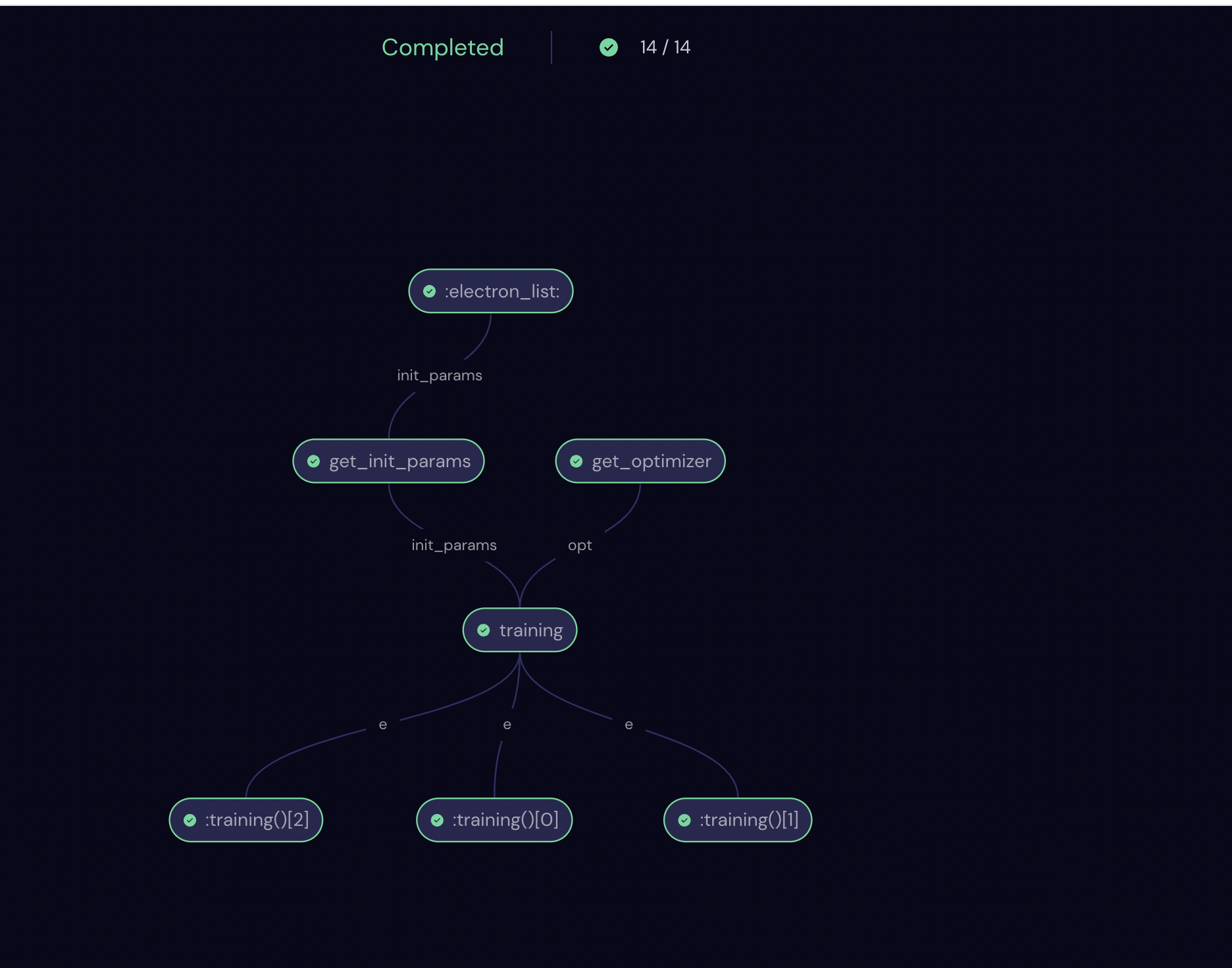
We can go to the Covalent UI at http://localhost:48008 to see a visual representation of the workflow we created as well as other information such as Input, Result, Executor, etc. In this particular case, our workflow looks like the following.
Now from the result we can see if the training was successful by tracking how the cost evolved with the training steps.
[7]:
fig, ax = plt.subplots(1, 1, figsize=(7, 5), facecolor="w")
ax.plot(traing_steps, cost_steps)
ax.set_xlabel("Training steps")
ax.set_ylabel("Cost")
ax.set_title("Cost vs. Training steps")
plt.tight_layout()
plt.show()
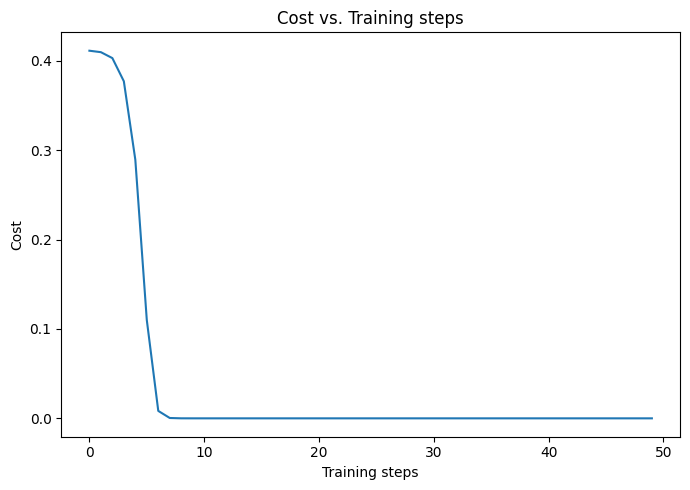
We see that the cost gets very close to zero in less than 10 training steps, indicating that the optimization was successful. Indeed, we can compare the expected photon number evaluated with the optimal parameters and the expectation value from the qubit circuit.
[8]:
print(photon_redirection(opt_params))
print(qubit_rotation(0.4, 0.8))
0.6417093721057024
0.6417093742397795
Summary#
In this tutorial we demonstrated how to use Covalent in conjuction with PennyLane for a hybrid task. Despite the simplicity of the task, the workflow should generalize straightforwardly to more complex tasks which can take advantage of the features of Covalent such as auto-parallelization and intelligent scheduling.