Classical and quantum support vector machines#
In this tutorial, we use Covalent to orchestrate a workflow that compares the perfomance of the SVM and QSVM models. We use the scikit-learn package for SVM and qiskit_machine_learning for QSVM implementations.
Covalent is responsible for:
constructing subtasks.
constructing workflows, which, are comprised of subtasks.
submitting the workflow for execution.
polling the execution status of individual subtasks and the workflow.
collecting the final results corresponding to the subtasks and the workflow.
First, we import all the packages related to plotting and constructing the SVM and QSVM models. scikit-learn is used to load a toy dataset for this tutorial.
[1]:
with open("./requirements.txt", "r") as file:
    for line in file:
        print(line.rstrip())
covalent
qiskit==0.36.0
qiskit-machine-learning==0.3.1
scikit-learn==1.0.2
matplotlib==3.6.3
[2]:
# Installing required packages
# !pip install -r ./requirements.txt
[3]:
# Import plotting library
import matplotlib.pyplot as plt

# Set global plot background color
plt.rcParams["figure.facecolor"] = "w"

# Import for SVM classifier
from sklearn.svm import SVC

# Imports for dataset and model selection
from sklearn import datasets
from sklearn.model_selection import train_test_split
from sklearn.metrics import ConfusionMatrixDisplay, confusion_matrix

# Imports for QSVC classifier
from qiskit import BasicAer
from qiskit.circuit.library import ZZFeatureMap
from qiskit.utils import QuantumInstance, algorithm_globals
from qiskit_machine_learning.kernels import QuantumKernel

# Set the random seed for QSVC
seed = 12345
algorithm_globals.random_seed = seed
Next, we import covalent to construct and manage our workflows.
[4]:
# Import workflow management library
import covalent as ct
The workflow is broken down into subtasks in order to compare the performance of SVM and QSVM. The list of subtasks are:
get_data- Retrieve a dataset commonly used for toy ML problems.split_train_test_data- Split the data into training and test subsets.train_svc- Train the SVC model with a classical linear kernel.train_qsvc- Train the QSVC model with a quantum kernel using theqiskitlibrary (more detailed tutorial here).
The subtasks are constructed using the ct.electron decorator.
[5]:
@ct.electron
def get_data():
    iris = datasets.load_iris()
    X = iris.data[:, :2]  # we only take the first two features.
    y = iris.target
    return X, y


@ct.electron
def split_train_test_data(X, y):
    X_train, X_test, y_train, y_test = train_test_split(X, y, test_size=0.25, random_state=0)
    return X_train, X_test, y_train, y_test


@ct.electron
def train_svc(X_train, y_train):
    svc = SVC(kernel="linear")
    svc.fit(X_train, y_train)
    return svc


@ct.electron
def train_qsvc(X_train, y_train):
    feature_map = ZZFeatureMap(feature_dimension=2, reps=2, entanglement="linear")
    backend = QuantumInstance(
        BasicAer.get_backend("qasm_simulator"), shots=16, seed_simulator=seed, seed_transpiler=seed
    )
    kernel = QuantumKernel(feature_map=feature_map, quantum_instance=backend)
    qsvc = SVC(kernel=kernel.evaluate)
    qsvc.fit(X_train, y_train)
    return qsvc
Having constructed the subtasks, we can now construct the workflow using the ct.lattice decorator.
[6]:
@ct.lattice
def workflow():
    X, y = get_data()
    X_train, X_test, y_train, y_test = split_train_test_data(X=X, y=y)
    svc_model = train_svc(X_train=X_train, y_train=y_train)
    qsvc_model = train_qsvc(X_train=X_train, y_train=y_train)
    return X_test, y_test, svc_model, qsvc_model
Note
It is important to provide the argument names in the electron definitions. train_svc(X_train, y_train) will raise an error while train_svc(X_train=X_train, y_train=y_train) will not. Additionally, note that we should create electrons to perform subtasks rather than manipulating objects inside the lattice.
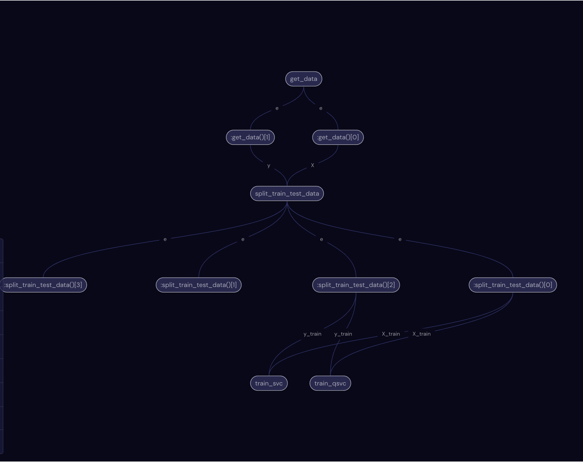
Next, we can visualize the workflow using the draw method. The visualization allows us to check if the workflow has been properly defined as well as retrieving the node ids corresponding to each subtasks.
Tip
The node ids are useful for retrieving the subtask execution details.
[7]:
workflow.draw()
One you run the above codeblock, you can check out the ui preview (default at localhost:48008/preview) and see the generated graph which will look like this:
[8]:
from IPython import display

display.Image("assets/workflow.png")
[8]:
Once we have ensured that the workflow has been constructed properly, we can submit the task via the dispatch method.
[9]:
dispatch_id = ct.dispatch(workflow)()
The execution result can be retrieved using the ct.get_result method.
Note
If we set wait=True, the method will wait for all the subtasks to finish executing before retrieving the final result. Otherwise, the method will return a result object that can be queried for execution status using the result.get_node_result(node_id) method.
[10]:
result = ct.get_result(dispatch_id=dispatch_id, wait=True)
[11]:
X_test, y_test, svc_model, qsvc_model = result.result
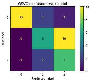
Once the computations is completed, we can plot the confusion matrix for the models as shown below.
[12]:
svc_cm_plot = ConfusionMatrixDisplay.from_estimator(svc_model, X_test, y_test)
svc_cm_plot.ax_.set_title("SVC confusion matrix plot")
[12]:
Text(0.5, 1.0, 'SVC confusion matrix plot')

[13]:
qsvc_cm_plot = ConfusionMatrixDisplay.from_estimator(qsvc_model, X_test, y_test)
qsvc_cm_plot.ax_.set_title("QSVC confusion matrix plot")
[13]:
Text(0.5, 1.0, 'QSVC confusion matrix plot')
Conclusion#
In this tutorial, we used covalent to construct a workflow to compare the performance of SVM and QSVM models. Note that the SVM model training requires a classical hardware while the QSVM model training requires quantum hardware. A primary benefit of covalent is the convenience with which computational jobs can be submitted to either classical or quantum hardwares.