MNIST classifier tutorial

MNIST database of handwritten digits is a popular dataset to demonstrate machine learning classifiers. The dataset is comprised of handwritten digits with the corresponding ground truth label. In this tutorial (based on [1]), we train a basic Neural Network (NN) classifier using PyTorch.

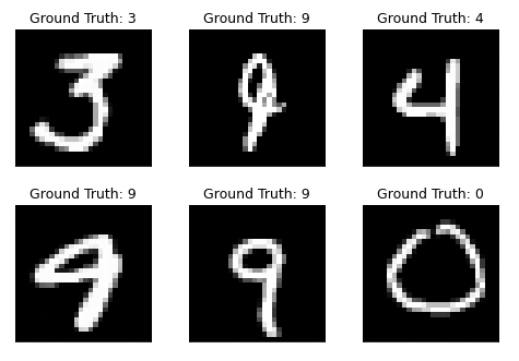
A sample of the MNIST dataset:

The tutorial has two main parts:

• First, a “normal” workflow function (without using Covalent) is defined to train the MNIST classifier.

• Second, this workflow is converted into a Covalent workflow, which is then “dispatched” for execution.

Lastly, we review the key benefits that are unlocked when transforming a “normal” workflow with Covalent. One major advantage of a Covalent workflow is that the task dependencies and execution details can be tracked easily in the Covalent user interface (UI).

Getting started

This tutorial requires installing Covalent, PyTorch and Torchvision.

with open("./requirements.txt", "r") as file:
    for line in file:
        print(line.rstrip())

covalent
torch==1.13.1
torchvision==0.14.1

Uncomment and run the following cell to install the libraries.

# Installing required packages
# !pip install -r ./requirements.txt

# In some cases, the following two lines might also need to be run
# !jupyter nbextension enable --py widgetsnbextension

Once Covalent has been installed, run covalent start in a terminal to start the Covalent server. Also, covalent status / stop are used to check the server status / stop the server.

Import Covalent, PyTorch and other relevant libraries.

import covalent as ct

import torch
import torch.nn.functional as F

from pathlib import Path

from torch import nn
from torch.utils.data import DataLoader
from torchvision import datasets
from torchvision.transforms import ToTensor
from typing import Tuple

Construct MNIST classifier training workflow (without Covalent)

Construct a convolutional neural network model by inheriting from torch.nn.Module.

class NeuralNetwork(nn.Module):
    def __init__(self):
        super(NeuralNetwork, self).__init__()
        self.conv1 = nn.Conv2d(1, 10, kernel_size=5)
        self.conv2 = nn.Conv2d(10, 20, kernel_size=5)
        self.conv2_drop = nn.Dropout2d()
        self.fc1 = nn.Linear(320, 50)
        self.fc2 = nn.Linear(50, 10)

    def forward(self, x):
        x = F.relu(F.max_pool2d(self.conv1(x), 2))
        x = F.relu(F.max_pool2d(self.conv2_drop(self.conv2(x)), 2))
        x = x.view(-1, 320)
        x = F.relu(self.fc1(x))
        x = F.dropout(x, training=self.training)
        x = self.fc2(x)
        return F.log_softmax(x, dim=1)

Construct a data loader to retrieve the classifier training and test data.

def data_loader(
    batch_size: int,
    train: bool,
    download: bool = True,
    shuffle: bool = True,
    data_dir: str = "~/data/mnist/",
) -> torch.utils.data.dataloader.DataLoader:
    """MNIST data loader."""

    data_dir = Path(data_dir).expanduser()
    data_dir.mkdir(parents=True, exist_ok=True)

    data = datasets.MNIST(data_dir, train=train, download=download, transform=ToTensor())

    return DataLoader(data, batch_size=batch_size, shuffle=shuffle)

Construct a function to retrieve a Stochastic Gradient Descent optimizer.

def get_optimizer(
    model: NeuralNetwork, learning_rate: float, momentum: float
) -> torch.optim.Optimizer:
    """Get Stochastic Gradient Descent optimizer."""

    return torch.optim.SGD(model.parameters(), learning_rate, momentum)

Write a function to train the model over one epoch.

def train_over_one_epoch(
    dataloader: torch.utils.data.dataloader.DataLoader,
    model: NeuralNetwork,
    optimizer: torch.optim.Optimizer,
    log_interval: int,
    epoch: int,
    loss_fn,
    train_losses: list,
    train_counter: int,
    device: str = "cpu",
):
    """Train neural network model over one epoch."""

    size = len(dataloader.dataset)
    model.train()
    for batch, (X, y) in enumerate(dataloader):
        X, y = X.to(device), y.to(device)

        # Compute prediction error
        pred = model(X)
        loss = loss_fn(pred, y)

        # Backpropagation
        optimizer.zero_grad()
        loss.backward()
        optimizer.step()

        if batch % log_interval == 0:
            loss, current = loss.item(), batch * len(X)
            print(f"loss: {loss:>7f}  [{current:>5d}/{size:>5d}]")

            train_losses.append(loss)
            train_counter.append((batch * 64) + ((epoch - 1) * len(dataloader.dataset)))

    return model, optimizer

Write a function to test the performance of the classifier for a given loss function.

def test(
    dataloader: torch.utils.data.dataloader.DataLoader,
    model: NeuralNetwork,
    loss_fn: callable,
    device: str = "cpu",
) -> None:
    """Test the model performance."""

    size = len(dataloader.dataset)
    num_batches = len(dataloader)
    model.eval()
    test_loss, correct = 0, 0
    with torch.no_grad():
        for X, y in dataloader:
            X, y = X.to(device), y.to(device)
            pred = model(X)
            test_loss += loss_fn(pred, y).item()
            correct += (pred.argmax(1) == y).type(torch.float).sum().item()
    test_loss /= num_batches
    correct /= size
    accuracy = 100 * correct
    print(f"Test Error: \n Accuracy: {(accuracy):>0.1f}%, Avg loss: {test_loss:>8f} \n")
    return accuracy, test_loss

Write a function to train the model over several epochs and save the final state of the optimizer and the neural network.

def train_model(
    train_dataloader: torch.utils.data.dataloader.DataLoader,
    train_losses: list,
    train_counter: int,
    log_interval: int,
    model: NeuralNetwork,
    learning_rate: float,
    momentum: float,
    loss_fn: callable,
    epochs: int,
    results_dir: str = "~/data/mnist/results/",
) -> Tuple[NeuralNetwork,]:
    """Train neural network model."""

    results_dir = Path(results_dir).expanduser()
    results_dir.mkdir(parents=True, exist_ok=True)

    optimizer = torch.optim.SGD(model.parameters(), learning_rate, momentum)
    for epoch in range(1, epochs + 1):
        print(f"Epoch {epoch}\n-------------------------------")
        model, optimizer = train_over_one_epoch(
            dataloader=train_dataloader,
            model=model,
            optimizer=optimizer,
            train_losses=train_losses,
            train_counter=train_counter,
            log_interval=log_interval,
            epoch=epoch,
            loss_fn=loss_fn,
        )

    # Save model and optimizer
    torch.save(model.state_dict(), f"{results_dir}model.pth")
    torch.save(optimizer.state_dict(), f"{results_dir}optimizer.pth")
    return model, optimizer

Finally, we put all these tasks together to construct the MNIST classifier training and test workflow.

def workflow(
    model: NeuralNetwork,
    epochs: int = 2,
    batch_size_train: int = 64,
    batch_size_test: int = 1000,
    learning_rate: float = 0.01,
    momentum: float = 0.5,
    log_interval: int = 200,
    loss_fn: callable = F.nll_loss,
):
    """MNIST classifier training workflow"""

    train_dataloader = data_loader(batch_size=batch_size_train, train=True)
    test_dataloader = data_loader(batch_size=batch_size_test, train=False)

    train_losses, train_counter, test_losses = [], [], []
    model, optimizer = train_model(
        train_dataloader=train_dataloader,
        train_losses=train_losses,
        train_counter=train_counter,
        log_interval=log_interval,
        model=model,
        learning_rate=learning_rate,
        momentum=momentum,
        loss_fn=loss_fn,
        epochs=epochs,
    )
    accuracy, test_loss = test(dataloader=test_dataloader, model=model, loss_fn=loss_fn)

    return accuracy, test_loss

Run MNIST classifier workflow as a normal function (without Covalent)

Run the MNIST classifier workflow to benchmark the performance and the time taken to train and test the model.

import time

start = time.time()
workflow(
    model=NeuralNetwork().to("cpu"),
)
end = time.time()

Epoch 1
-------------------------------
loss: 2.294023  [    0/60000]
loss: 2.269915  [12800/60000]
loss: 1.836730  [25600/60000]
loss: 1.027309  [38400/60000]
loss: 0.857166  [51200/60000]
Epoch 2
-------------------------------
loss: 0.509862  [    0/60000]
loss: 0.667653  [12800/60000]
loss: 0.735403  [25600/60000]
loss: 0.497471  [38400/60000]
loss: 0.439544  [51200/60000]
Test Error:
 Accuracy: 93.9%, Avg loss: 0.195917

print(f"Regular workflow takes {end - start} seconds.")

Regular workflow takes 31.566487073898315 seconds.

The final test accuracy is 93.5% and average loss is 0.211207.

Transform and run workflow with Covalent

First, we convert the normal workflow function into a Covalent workflow function.

This can be done in two ways. The most convenient method is to add ct.electron decorators to each of the task functions defined above and ct.lattice decorator to the workflow function.

For example,

@ct.electron
def data_loader(...):
    ...


@ct.electron
def train_over_one_epoch(...):
    ...


@ct.lattice
def workflow(...):
    ...

Alternatively, we can also use the decorator functions (shown in the cell below):

# Convert tasks to electrons
data_loader = ct.electron(data_loader)
get_optimizer = ct.electron(get_optimizer)
train_over_one_epoch = ct.electron(train_over_one_epoch)
train_model = ct.electron(train_model)
test = ct.electron(test)

# Convert workflow to lattice
workflow = ct.lattice(workflow, executor="local")

Note: We use the “local” executor in this tutorial because the default Dask-based executor does not yet capture the output of print statements. This issue will be addressed in a future release.

Finally, Covalent dispatcher (ct.dispatch) can be used to dispatch the workflow.

dispatch_id = ct.dispatch(workflow)(model=NeuralNetwork().to("cpu"))
print(f"Dispatch id: {dispatch_id}")
result = ct.get_result(dispatch_id=dispatch_id, wait=True)
print(f"Covalent workflow takes {result.end_time - result.start_time} seconds.")
print(f"Covalent workflow execution status: {result.status}")

Dispatch id: 37dfe2e9-b477-4282-b695-f7850a9f95a3
Covalent workflow takes 0:00:40.219979 seconds.
Covalent workflow execution status: COMPLETED

To view a summary of the result object, uncomment and run the following cell.

# print(result)

print(result.get_node_result(6)["stdout"])

Epoch 1
-------------------------------
loss: 2.280812  [    0/60000]
loss: 2.257816  [12800/60000]
loss: 1.388549  [25600/60000]
loss: 0.865922  [38400/60000]
loss: 0.636836  [51200/60000]
Epoch 2
-------------------------------
loss: 0.723659  [    0/60000]
loss: 0.648925  [12800/60000]
loss: 0.440847  [25600/60000]
loss: 0.445998  [38400/60000]
loss: 0.331685  [51200/60000]

print(result.get_node_result(19)["stdout"])

Test Error:
 Accuracy: 93.8%, Avg loss: 0.213674

Once the workflow has been dispatched, the results can be tracked on the Covalent UI. Use covalent status (shown below) to find the browser address to access the Covalent UI.

!covalent status

Covalent server is running at http://localhost:48008.

Clicking on http://localhost:48008 we can see the Covalent UI which lists the various dispatch ids.

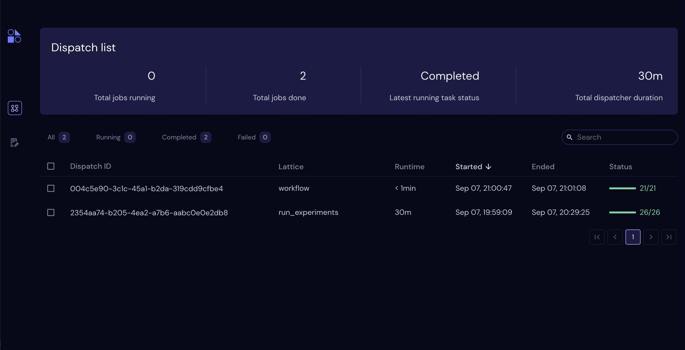
Clicking on the dispatch id, we can see the details of the workflow execution. Note the task execution dependency graph.

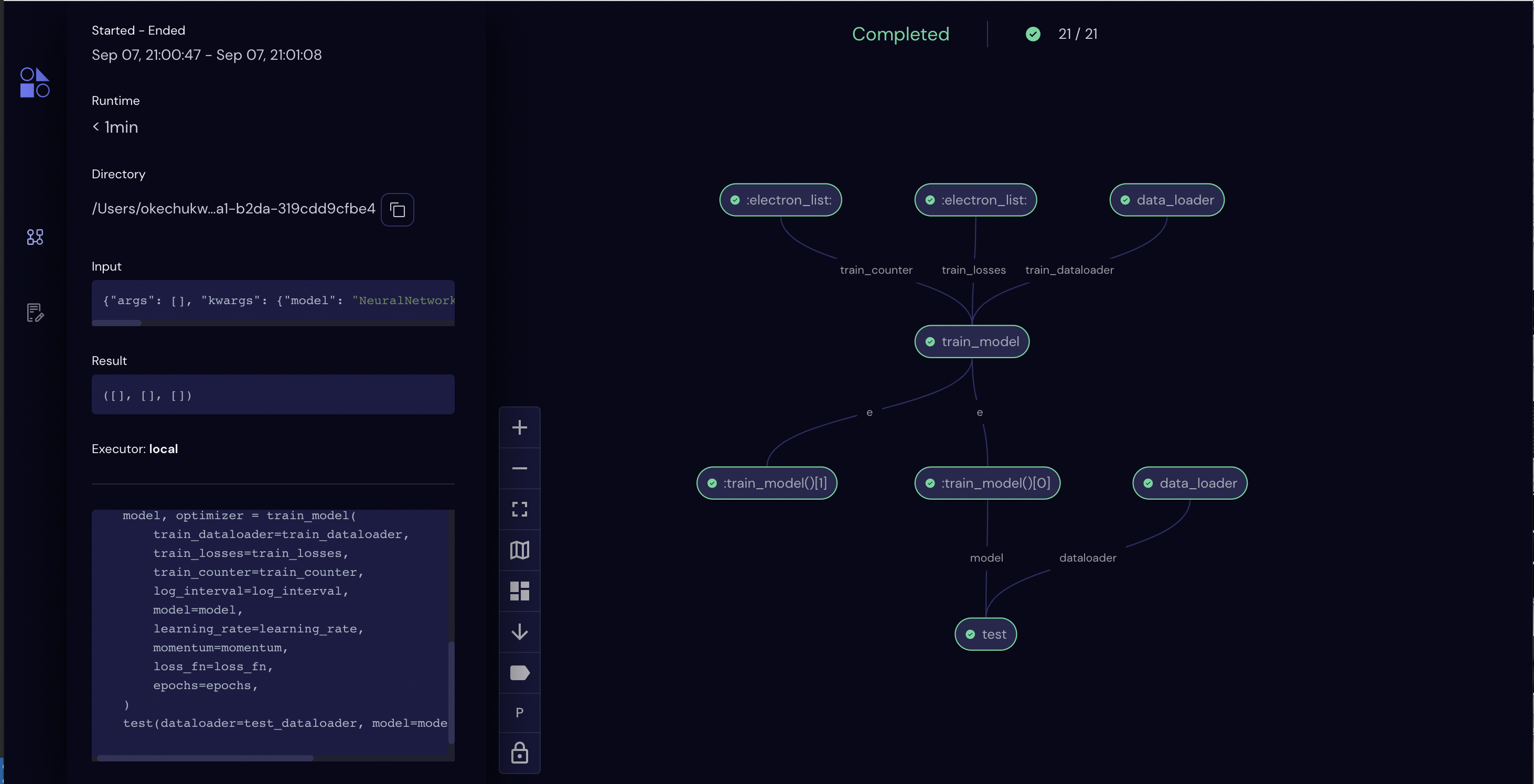
Furthermore, the progress and status of the tasks (get_optimizer, data_loader etc.) can also be tracked in the Covalent UI.

Conclusion

In this tutorial, we trained a MNIST classifier using a workflow comprised of several tasks. Then, we converted this workflow into a Covalent workflow. Here, we summarize some of the added benefits of using Covalent.

• Covalent allows the user to deploy multiple workflows without having to wait for them to finish running. This makes it very useful for experimentation in a pre-production environment.

• A Covalent workflow can be dispatched to take advantage of automatic parallelization, user friendly interface etc. but it can also just as easily be run as a normal Python function. Hence, adding the electron / lattice decorators only enhances what can be done with the workflow with a minimum work. For example, in this workflow the training and testing of dataloaders (I/O bound tasks) are mutually independent and hence would be automatically parallelized.

• Execution time for Covalent workflows and tasks are readily available without needing any additional code.

• In this tutorial, we saw that the execution time overhead added by Covalent is small (10 seconds) and scales very well as the problems grow in complexity. Particularly for problems that are parallelizable, Covalent becomes a much better alternative than a regular workflow.

References:

[1] https://pytorch.org/tutorials/beginner/basics/quickstart_tutorial.html